グラフ結果
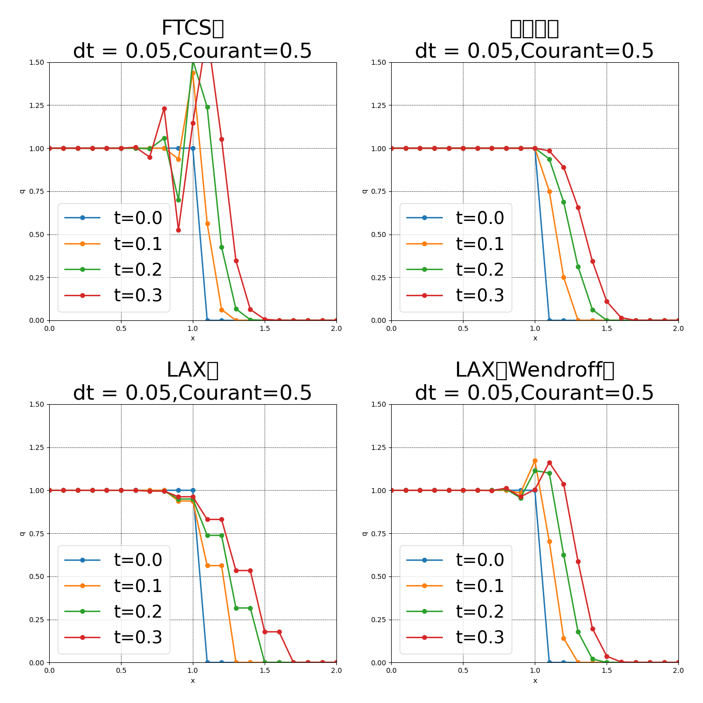
CFL = 0.5 での計算結果。FTCS は発散、風上差分・Lax は数値拡散、Lax-Wendroff は2次精度だが不連続付近に振動が見られる。
1次元移流方程式を4種類の差分法で数値的に解き、各手法の安定性・精度・拡散性を2×2のサブプロットで比較するコード。
| 項目 | 内容 |
|---|---|
| 対象方程式 | 1次元移流方程式 ∂q/∂t + c ∂q/∂x = 0 |
| 移流速度 | c = 1 |
| 空間刻み | dx = 0.10(格子点数 jmax = 21) |
| 時間刻み | dt = 0.05(ステップ数 nmax = 600) |
| CFL数 | ν = c·dt/dx = 0.5 |
| 初期条件 | ステップ関数(x < 1 で q=1、x ≥ 1 で q=0) |
| 出力時刻 | t = 0.1, 0.2, 0.3 |
| 比較手法 | FTCS法 / 風上差分 / Lax法 / Lax-Wendroff法 |
| ライブラリ | 用途 |
|---|---|
numpy | 配列演算・初期条件の設定 |
matplotlib.pyplot | 2×2サブプロットへの描画 |
日本語フォントを明示的に指定:
plt.rcParams['font.family'] = 'IPAexGothic'未インストールの場合は sudo apt install fonts-ipafont -y で導入する。
1次元移流方程式は流体の移流現象を最もシンプルに記述した方程式で、解析解はステップ波形が速度 c で平行移動するものとなる:
数値解法ではこの「形を保って移動する」挙動を再現できるかが精度の指標となる。 拡散・振動・不安定化のいずれが生じるかは差分スキームの特性に依存し、本コードはその違いを視覚的に比較する。
時間:前進差分(1次精度)、空間:中心差分(2次精度)。 ただし von Neumann 安定性解析よりCFL ≤ 1 でも無条件不安定。波形が時間とともに振動・発散する。
時間:前進差分(1次精度)、空間:後退差分(1次精度)。c > 0 のとき CFL ≤ 1 で条件付き安定。 数値拡散が生じ、ステップ波形が滑らかになる。精度は時間・空間ともに1次。
FTCSの q[j]ⁿ を隣接点の平均 (q[j+1]ⁿ + q[j-1]ⁿ)/2 に置き換えたスキーム。
CFL ≤ 1 で安定だが、数値拡散が大きく、波形の鋭い不連続が大きく広がる。精度は1次。
テイラー展開で2次の項まで取り込んだスキーム。時間・空間ともに2次精度。CFL ≤ 1 で安定。 数値拡散は小さいが、不連続付近に数値振動(リンギング)が生じる。
q_init を作成(x<1 で q=1、x≥1 で q=0)n*dt が plot_times に一致するステップで描画plt.tight_layout() でレイアウト整形して出力境界条件:j = 1 ~ jmax-2 のみ更新(両端 j=0, j=jmax-1 は固定値のまま)。
| スキーム | 空間精度 | 時間精度 | 安定条件 | 特徴 |
|---|---|---|---|---|
| FTCS | 2次 | 1次 | 無条件不安定 | 振動・発散 |
| 風上差分 | 1次 | 1次 | CFL ≤ 1 | 数値拡散大 |
| Lax | 1次 | 1次 | CFL ≤ 1 | 数値拡散大(最大) |
| Lax-Wendroff | 2次 | 2次 | CFL ≤ 1 | 数値振動(リンギング) |
本コードの設定は CFL = 0.5 なので、FTCS 以外の3手法は安定。
import numpy as np
import matplotlib.pyplot as plt

c=1
#dt=0.05

fig, axes = plt.subplots(2, 2, figsize=(14, 14), dpi=100)
plt.rcParams["font.size"]=25
plt.rcParams['font.family'] = 'IPAexGothic'

dt=0.05
dx=0.10
jmax=21
nmax=600
plot_times = [0.1, 0.2, 0.3]
x=np.linspace(0,dx*(jmax-1),jmax)
q_init=np.zeros(jmax)
for j in range(jmax):
   if(j<jmax/2):
       q_init[j]=1
   else:
       q_init[j]=0

#***FTCS**********************************************************
ax=axes[0,0]
q=q_init.copy()
ax.plot(x,q,marker='o',lw=2,label='t=0.0')
for n in range(1,1+nmax):
    qold=q.copy()
    for j in range(1,jmax-1):
        q[j]=qold[j]-dt*c*(qold[j+1]-qold[j-1])/(2*dx)
    if any(np.isclose(n*dt, pt) for pt in plot_times):
        ax.plot(x,q,marker='o',lw=2,label=f't={n*dt:.2g}')
ax.grid(color='black',linestyle='dashed',linewidth=0.5)
ax.set_xlabel('x'); ax.set_ylabel('q')
ax.set_xlim([0,2]); ax.set_ylim([0,1.5])
ax.set_title(f'FTCS法\ndt = {dt},Courant={dt*c/dx:.2g}')
ax.legend()

#***風上差分**********************************************************
ax=axes[0,1]
q=q_init.copy()
ax.plot(x,q,marker='o',lw=2,label='t=0.0')
for n in range(1,1+nmax):
    qold=q.copy()
    for j in range(1,jmax-1):
        q[j]=qold[j]-dt*c*(qold[j]-qold[j-1])/(dx)
    if any(np.isclose(n*dt, pt) for pt in plot_times):
        ax.plot(x,q,marker='o',lw=2,label=f't={n*dt:.2g}')
ax.grid(color='black',linestyle='dashed',linewidth=0.5)
ax.set_xlabel('x'); ax.set_ylabel('q')
ax.set_xlim([0,2]); ax.set_ylim([0,1.5])
ax.set_title(f'風上差分\ndt = {dt},Courant={dt*c/dx:.2g}')
ax.legend()

#***LAX***********************************************************
ax=axes[1,0]
q=q_init.copy()
ax.plot(x,q,marker='o',lw=2,label='t=0.0')
for n in range(1,1+nmax):
    qold=q.copy()
    for j in range(1,jmax-1):
        q[j]=1/2*(qold[j+1]+qold[j-1])-dt*c/2*(qold[j+1]-qold[j-1])/(dx)
    if any(np.isclose(n*dt, pt) for pt in plot_times):
        ax.plot(x,q,marker='o',lw=2,label=f't={n*dt:.2g}')
ax.grid(color='black',linestyle='dashed',linewidth=0.5)
ax.set_xlabel('x'); ax.set_ylabel('q')
ax.set_xlim([0,2]); ax.set_ylim([0,1.5])
ax.set_title(f'LAX法\ndt = {dt},Courant={dt*c/dx:.2g}')
ax.legend()

#***LAX-Wendroff***********************************************************
ax=axes[1,1]
q=q_init.copy()
ax.plot(x,q,marker='o',lw=2,label='t=0.0')
for n in range(1,1+nmax):
    qold=q.copy()
    for j in range(1,jmax-1):
        q[j]=qold[j]-dt*c/2*(qold[j+1]-qold[j-1])/(dx)+(dt*c)**2/2*(qold[j+1]-2*qold[j]+qold[j-1])/(dx)**2
    if any(np.isclose(n*dt, pt) for pt in plot_times):
        ax.plot(x,q,marker='o',lw=2,label=f't={n*dt:.2g}')
ax.grid(color='black',linestyle='dashed',linewidth=0.5)
ax.set_xlabel('x'); ax.set_ylabel('q')
ax.set_xlim([0,2]); ax.set_ylim([0,1.5])
ax.set_title(f'LAXーWendroff法\ndt = {dt},Courant={dt*c/dx:.2g}')
ax.legend()

plt.tight_layout()
plt.show()CFL = 0.5 での計算結果。FTCS は発散、風上差分・Lax は数値拡散、Lax-Wendroff は2次精度だが不連続付近に振動が見られる。